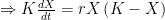
Looking south to the upper Gulf of California and the Colorado River delta
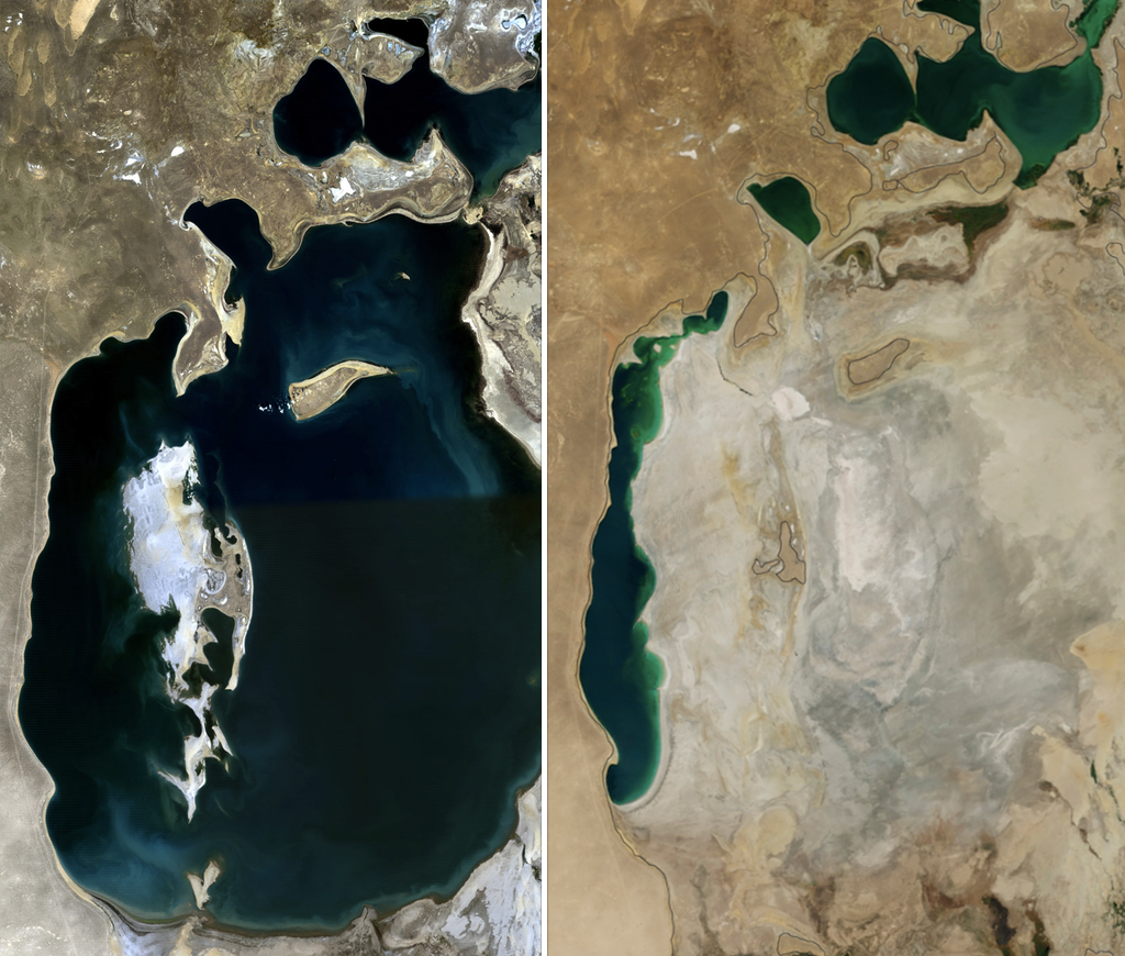
Many years ago, in the late 1990’s, I had the privilege and pleasure of working with Karl Flessa at the University of Arizona. I had gone there as a researcher to participate in Karl’s Gulf of California project, as one component of the project involved a group of marine bivalves (clams) on which I was an expert. The goal of the project was to assess the changes that had taken place, and were ongoing, in the northern Gulf after damming of the Colorado River. By the time that we were working there, it had been several decades since freshwater flowed into the former river delta in any appreciable volume. Almost all the water, which is generated largely from snowmelt in the Rocky Mountains, is now utilized by the western United States and Mexico. The changes were profound; increases of salinity, increased tidal influence, changes of dominant species and so on, much of which has been documented by the aptly named CEAM (El Centro de Estudios de Almejas Muertas). This was my first introduction to the then nascent field of conservation paleobiology, which has since developed into a major subdiscipline of the paleobiological sciences. The community is now centered around the Conservation Paleobiology Network, a great resource for learning more. The goal of conservation paleobiology is to apply paleontological and geological work, primarily of past species and ecological systems, to understanding, conserving, and regenerating current ecological systems.
Roxanne Banker, Scott Sampson and I published a conservation paleobiology paper last year in which we proposed a new approach to both conservation biology and paleobiology, the Past-Present-Future (PPF) strategy. The idea is to use conservation paleobiology as a rubric to combine diverse data streams, e.g. fossils, historical data, indigenous knowledge, with mathematical modeling to reconstruct historical and current systems, and apply the results to conservation in the near-term future. The paper focused on the role of an extinct sirenian (manatees, dugongs), Steller’s Sea Cow, in the dynamics of North Pacific giant kelp forests. Those forests have been devastated during the past decade by marine heat waves, and the loss of sunflower sea stars, a major predator of the kelp-consuming purple sea urchin. We found that kelp forests would have, under many circumstances, been more resilient to those disturbances in the presence of the sea cow. Unfortunately, the sea cow was driven (consumed) to extinction in the early to mid-18th century, shortly after its discovery by Russian commercial hunters.
Recently Scott and I have published an opinion piece in Scientific American magazine, We Need to Think about Conservation on a Different Timescale, in which we more broadly advocate for the PPF approach and conservation paleobiology. The mathematical modeling of historical and ancient ecosystems can be extremely challenging, but as we showed in our paper, and argue in this opinion article, it is both feasible and bears great potential. As we state in the closing of the article: “We are all characters in an epic story that has been unfolding for millions upon millions of years. The decisions we make today will shape how the future unfolds. It’s high time we embraced our role in this ever-evolving drama and established vital through lines from past to future.“
I just received an interesting query from a journalist who is working on the apparently imminent collapse of the Sonoran Desert ecosystem. The question was, “Why does it matter if the Sonoran ecosystem collapses?” I found this to be very interesting because, in contrast to “what does ecosystem collapse mean”, the question was about why it matters. This is a very good question as potentially takes us beyond the scientific meaning, and is asking more broadly, why should we care? I realized that I actually don’t have a certain answer for this, but I tried to provide a brief and thoughtful response, which I now include here…
“Well, that’s actually a very good question. There’s a difference I guess between what it means, and why it matters. I’ll give you my take on it.
An ecosystem is something that humans define (e.g. see https://www.cambridge.org/core/books/ecosystem-functioning/148A9BB94FCCFD3F4AE23B675FB6511E), generally as the assemblage of species and their environment in a particular place, and at a particular time. An ecosystem is collectively all those species and their interactions with each other and the environment, and the processes that emerge from those interactions. It is the processes, such as energy flow or nitrogen fixation, that sustain the system. So there is this feedback loop, where species create processes, and the collection of those processes create the conditions necessary for the species to persist. The collapse of an ecosystem is a breakdown of that loop, where because of species losses or environmental changes, or both, some species no longer contribute to a particular process, or a process that is necessary for the persistence of a species is no longer sufficient or present. The result is a disruption of species functioning, accompanied by the decline or extinction of species, and a disruption of environmental processes.
Why does that matter if the Sonoran system collapsed? I think that it depends a bit on who you ask. It matters from the biodiversity perspective, because of the loss or increased risk of loss of species. Many people place great value on the intangible value of biodiversity. Biodiversity is the foundation of ecosystem resilience, and changes to that biodiversity changes ecosystem resilience. And resilient ecosystems provide ecosystem services, which are the benefits that human societies gain from ecosystem functioning, such as oxygen, clean water, biological resources, etc. So in addition to the loss of a rather unique system of species, and their evolutionary potentials/futures, we will also reduce the benefits that societies connected to the Sonoran system are dependent upon. And that is a cascading consequence, of course, as those societies then will look elsewhere for those benefits.”
Yuangeng Huang was a recent post-doctoral researcher in my lab at the California Academy of Sciences. Several years ago, while conducting his Ph.D. research at the China University of Geosciences (CUG) in Wuhan, Yuangeng trekked over to the United States and spent about six months in my lab, where he learned a great deal about the sorts of paleoecological modeling that we do. Then after completing his Ph.D., he joined me in my lab in the fall of 2019 as a post-doc. This was ideal, as part of Yuangeng’s dissertation research was on late Paleozoic and early Mesozoic terrestrial faunas from the Xinjiang region of China, which coincided with a large collaborative project in the Integrated Earth Systems program at the US NSF, of which I am a part. Yuangeng and I had great plans for the coming year, but of course 2020 was anything but a normal year. Unfortunately Yuangeng spent much of his time in the COVID-19 lockdown, along with most residents of the California Bay Area. Nevertheless, we adjusted as had so many other people around the world, and we did manage to do some very nice work, in my opinion. Yuangeng headed back to Wuhan in the fall of 2020 to take up a new position at CUG.
The first product of our time together is a recent paper published in the Royal Society Proceedings B, entitled “Ecological dynamics of terrestrial and freshwater ecosystems across three mid-Phanerozoic mass extinctions from northwest China“. In the paper we examined a span of 121 million years, comparing three mass extinctions: the end-Guadalupian event, the end Permian, and the Triassic-Jurassic transition. The end Permian mass extinction is by far the most severe recorded in the geological record. We compared the stabilities of terrestrial-aquatic communities within this span by reconstructing functional networks and food webs of the communities, and using mathematical models to subject them to disruptions of primary productivity (photosynthesis). The results of such perturbations are disruptions of populations, and eventually extinctions as the magnitude of the perturbations increases. What we found is that the two smaller events struck at times when communities were at relatively lower stability compared to the end Permian, but that recovery after the latter event was significantly more prolonged. This is yet a bit more evidence of the uniqueness of the end Permian extinction and the Permian-Triassic transition. Interestingly our results here are consistent with results for similar examinations of coeval communities from the Karoo Basin of South Africa, despite those communities being both taxonomically and ecologically different from the Xinjiang communities.
Comparing the stabilities of late Palezoic and early Mesozoic communities from northwest China (Huang et al., 2021). “Collapse threshold” is the point at which a community collapses when subjected to disruptions of primary productivity.
The paper is the result of a great collaboration, led by Yuangeng, involving researchers from China (including Yuangeng’s dissertation advisor, Zhong-Qiang Chen), the United States (including Wan Yang and myself), and the United Kingdom (Michael Benton). There are important communities from these times preserved elsewhere in the world (Russia, Brazil, Australia), giving us the potential to eventually truly understand the dynamics underlying these important events in biodiversity’s history.
WHAT IS ECOLOGICAL STABILITY? In 2019 I posed this question informally to colleagues, using Twitter, a professional workshop that I lead, and a conference. Respondents on Twitter consisted mostly of ecological scientists, but the workshop included paleontologists, biologists, physicists, applied mathematicians, and an array of social scientists, including sociologists, anthropologists, economists, archaeologists, political scientists, historians and others. And this happened…
In the previous post, we discussed the dramatic decline of the Atlantic cod (Gadus morhua) off Newfoundland over the past 60 years. I left us with the question of why, given the very limited catch sizes since the 1990’s, there was little evidence of population recovery (at least up until 2005). An Allee effect is a likely explanation for the failure of the population to recover during that extended period of reduced fishing pressure.
Beginning around 1994, the population may have become limited by an Allee phenomenon, or more appropriately mechanism, where a population’s size is limited far below the presumed carrying capacity, or observed maximum population size, because of reduced population size itself. Analogous to carrying capacity, where an upper limit is set on population growth rate by the effects of a relatively large population size, an Allee effect is an upper limit set by relatively small population size. Intuitive examples are easy to find, e.g. (1) species that require sufficient numbers for successful defense against predators will be increasingly limited by predation at low population size; (2) species for which habitat engineering by a sufficient number of individuals is necessary for offspring success; (3) species that depend on a minimum number of participants for the formation of successful mating assemblages. G. morhua, in which individual fecundity increases with age and body size (to a limit) (Fudge and Rose, 2008), is known to form, or have formed, large pelagic assemblages during spawning. Allee effects, therefore, describe situations where individual fitness depends on the presence of conspecifics, and is positively correlated with population size.
One vulnerability of populations subject to Allee effects is that small population size becomes an inescapable trap, with the likelihood of extinction increasing as population size declines. The reasons for this are twofold. First, if growth rates decline to zero or even become negative below an Allee threshold, then the state of zero population size becomes a stable state and extinction is assured. If you recall, our earlier models of population growth considered X= 0 (extinction) to be an unstable steady state; unstable because the addition of reproducing individuals to the population would result in divergence away from the zero state —population growth. Second, even if growth rate never becomes negative below the Allee threshold, a sufficiently large or sustained decline of population size increases the probability of extinction due to random events, a phenomenon termed stochastic extinction. Stochastic extinction, the probability of which could increase with deteriorating environmental conditions, is of interest to anyone studying extinction, including paleontologists, and will be discussed in a later section. Here, however, we will first explore several simple models of Allee effects.
Models of Allee effects
In the logistic model (Eq. 1 here), mortality rate increases as population size, X, approaches carrying capacity K, and population growth rate subsequently declines. The logistic model has two alternative steady states, X=K and X= 0, the latter of which is unstable as discussed above. The extinct state is a stable attractor, however, in the presence of an Allee effect. There are several simple models that demonstrate the effect, but to appreciate them, and the Allee effect itself, let us first examine the relationship between population size and growth rate under the logistic model. If we plot growth rate (dX/dt) against population size in the logistic model (Fig. 1), we see that the rate increases steadily at small population size, reaches a maximum when population size is half of the carrying capacity —X(t) =K/2— and declines steadily thereafter, reaching zero at carrying capacity. This value can be arrived at analytically because what we are visualizing is the rate of change of growth rate itself, technically the second derivative of the logistic growth equation. If we expand the logistic growth rate equation and take the derivative, we derive the acceleration (or deceleration) of the rate of change of population size as a function of population size itself. Setting d2X/dt equal to zero —the point at which growth rate is neither accelerating nor decelerating— we get the maximum that is illustrated in Fig. 1. The important thing to note here is that growth rate is always positive when 0<X(t)<K, that is, when population size lies between zero and the carrying capacity.
Fig. 1: The relationship between population growth rate and population size under a logistic model. In this example carrying capacity K=100.
There are several ways in which an Allee effect can be modelled in a logistically growing population. For example, if the Allee threshold is represented as a specific population size A, then the effect can be incorporated into the logistic formula as (Lewis and Kareiva, 1993; Boukal and Berec, 2002). The first term on the RHS of the equation is the logistic function, where growth declines to zero as X approaches K. The second term introduces the threshold, A, with growth rate declining if X < A, and increasing when X > A. Here, the effect is treated as the difference between population size and the threshold, taken as a fraction of carrying capacity, or maximum population size. Note that if A=0 —there is no Allee effect— the model reduces to the logistic growth model. A more nuanced model, where A must be greater than zero —an Allee effect always exists— treats the Allee threshold as equivalent yet opposite to K, representing a lower bound on growth rate (Courchamp et al., 1999). If A=1 —in which a population comprising a single individual is compromised under all circumstances— then the strength of the Allee effect depends on the size of the population. In both models, growth rate becomes negative below the threshold A, effectively dooming the population to extinction (Fig. 2). This condition is often termed a “strong” Allee effect.
Negative growth rates, a feature that is common to many models of the Allee effect, can be somewhat problematic from a conceptual viewpoint because of their determinism. We’ll pick this point up in the next post, and also discuss why paleontologists might care about both Allee effects, and model determinism.
Fig. 2: Two models of strong Allee effects illustrates as plots of population growth rate vs. population size. K=100. Red shows the first model where growth rate is relative to the Allee threshold A as a function of K. Blue shows the second model where growth rate is relative to the threshold A itself.
Vocabulary Allee effect — A positive correlation between individual fitness, or population growth rate, and population size. This means that fitness and/or growth rates decrease with declining population size. Second derivative — The derivative of a function’s derivative (the first derivative), thus the acceleration (deceleration) of a rate. E.g. the first derivative of a body in motion, described by position and time, is velocity or speed. The second derivative is acceleration, or the rate at which the speed is changing. Stochastic extinction — A relationship between the probability of a population’s extinction, and population size and/or environmental variability. In general, the risk of extinction increases due to random fluctuations of either factor. Strong Allee effect — Population growth rate becomes negative below some threshold of population size.
References Boukal, D. S. and Berec, L. (2002). Single-species models of the Allee effect: extinction boundaries, sex ratios and mate encounters. Journal of Theoretical Biology, 218(3):375–394. Courchamp, F., Clutton-Brock, T., and Grenfell, B. (1999). Inverse density dependence and the Allee effect. Trends in Ecology & Evolution, 14(10):405–410 Fudge, S. B. and Rose, G. A. (2008). Changes in fecundity in a stressed population: Northern cod (Gadus morhua) off Newfoundland. Resiliency of gadid stocks to fishing and climate change. Alaska Sea Grant, University of Alaska Fairbanks. Lewis, M. and Kareiva, P. (1993). Allee dynamics and the spread of invading organisms.Theoretical Population Biology, 43(2):141–158
WHAT IS ECOLOGICAL STABILITY ? In 2019 I posed this question informally to colleagues, using Twitter, a professional workshop that I lead, and a conference. Respondents on Twitter consisted mostly of ecological scientists, but the workshop included paleontologists, biologists, physicists, applied mathematicians, and an array of social scientists, including sociologists, anthropologists, economists, archaeologists, political scientists, historians and others. And this happened…
The Atlantic cod, Gadus morhua, has been the foundation of one of the world’s major fisheries for several centuries, with the Grand Banks off Newfoundland (Fig. 1) being amongst the most productive fisheries in the world. Figure 2 (below) shows the estimated population size of the Atlantic cod on the southern Grand Banks from the years 1959 to 2005 (Power et al., 2010), where G. morhua has historically been the most prominent component of that productive fishery. Cod populations, however, declined across the North Atlantic during the second half of the 20th century, most notably in the northwestern Atlantic. Several factors might have played roles, including warming ocean temperatures and a resurgence of the predatory grey seal across its historic range after implementation of protection from hunting (Neuenhoff et al., 2019). There is little doubt, however, that over-exploitation by commercial fisheries has been one of, if not the most effective driver of the decline. The Grand Banks population initially increased steadily during the monitored period, reaching a maximum in 1966. Thereafter it declined significantly until 1976, after which it appeared to stabilize, before beginning a steady decline in 1985. Fishing mortality of older individuals (> 6 years old) meanwhile fluctuated, peaking in 1975 and again in 1991. Change point analysis, which is used to detect changes in the statistical distribution of data within a time series, suggests that the population underwent significant shifts in 1971, 1985 and 1993. Each time, the mean population sizes of the intervals defined by those shifts descended through transient phases to significantly lower sizes. The first transition, around 1971, was preceded by an interval of highly variable population size, yet those sizes all exceeded population size from 1971 onward. The period from 1975-1985 was characterized by reduced population size and low variability, but another change occurred in 1985, and by 1993 the population size had stabilized at abysmally low numbers, marking the end of the commercially viable fishery.
Estimated population size (connected line) and fishery catch size (red) for the period 1959-2005. Arrows show times of presumed regime shifts, as identified by change point analysis.
It seems reasonable to hypothesize that each interval between the change point transitions represents a stable state or regime of the population, with fishing mortality thus driving or contributing to transitions between multiple alternative states (Fig. 2). The relationship between fishing and population size is relatively straightforward. Initially, an increase of total catch in the late 1960’s followed an increase of population size, but then declined as population size itself began a steep decline in 1967. However, although population size continued to decline, catch size again increased in 1971, coincident with the time marked by the change point analysis as the first transition to a state of smaller population size. Catch size subsequently followed the decline of population size, reaching a minimum during 1978, after which it began to increase again, presumably in response to the relatively “stable” population. Population size increased after 1980, reaching a new maximum in 1985, but then after a sharp increase of catch size, began its decline to the low numbers at the turn of the century.
A phase map (Fig. 3) captures this journey of potential alternative stable states and transitions, and reveals two general types of regime shifts. First, the initial transition to the second state that persisted from the late 1970s to 1985 was likely both precipitated and maintained by fishing pressure. The continued decline of catch size between 1971 and 1978 might have in fact facilitated some recovery of population size. This is the first type of regime shift and the separation of states—an external driver is capable of moving the system between states, and of maintaining the system in at least one of those states. The basic dynamics of this type of regime shift can be understood in terms of external parameters. The second type of shift, however, is less transparent, because it involves intrinsic properties and dynamics of the system. Look closely at the population trajectory from 1995 on, the last transition of the series. Catch size is negligible over a period of ten years, yet there is no sign of population rebound. If, as claimed earlier, population size is driven by catch size, why didn’t the population recover, and what kept it in the final, most recent attractor or state?
Phase map of cod population size, plotting consecutive years against each other. Blue trajectories show intervals of presumed population stability, i.e., stable states. Red trajectories show the pathways of transition between those states.
References Neuenhoff, R. D., Swain, D. P., Cox, S. P., McAllister, M. K., Trites, A. W., Walters, C. J., and Ham-mill, M. O. (2019). Continued decline of a collapsed population of Atlantic cod (Gadus morhua) due to predation-driven Allee effects. Canadian Journal of Fisheries and Aquatic Sciences, 76(1):168–184.
Power, D., Morgan, J., Murphy, E., Brattey, J., and Healey, B. (2010). An assessment of the cod stock in NAFO divisions 3NO. Northwest Atlantic Fisheries Organization SCR Doc, 10:42.
WHAT IS ECOLOGICAL STABILITY ? In 2019 I posed this question informally to colleagues, using Twitter, a professional workshop that I lead, and a conference. Respondents on Twitter consisted mostly of ecological scientists, but the workshop included paleontologists, biologists, physicists, applied mathematicians, and an array of social scientists, including sociologists, anthropologists, economists, archaeologists, political scientists, historians and others. And this happened…
Numerous terms, with roots across multiple disciplines that deal with dynamic complex systems, are used interchangeably in the study of transitions to some extent because they are related by process and implication. But they do not necessarily always refer to the same phenomena, and it is useful to be explicit in one’s usage (maybe at the risk of usage elsewhere). Regime shift, critical transition and tipping point are three of the more commonly applied terms in the ecological literature. They form a useful general framework within which to explore the concept of multiple states and transitions, and into which more detailed concepts can be introduced. Regime shift is defined here as an abrupt or rapid, and statistically significant change in the state of a system, such as a change of population size (Fig. 1A). Transient deviations or excursions from previous values, e.g. those illustrated in Fig. 1B}, are not regime shifts. “Regime” implies that the system has been observed to have remained at a stationary mean or within a range of variation over a period of time, and to then have shifted to another mean and range of variation. Regimes can be maintained by external or intrinsic processes, or sets of interacting external parameters and internal variables, but the ways in which the processes are organized can vary. Sets of processes can be dominant, reinforcing the regime; understanding this simply requires one to associate a regime with our previous discussions of system states and attractors. Regime shifts occur then when sets of processes are re-organized, and dominance or reinforcement shifts to other parameters and variables.
Fig. 1A – Hypothetical regime shift
Fig. 1B – Two populations of red-wing blackbirds. See here for an explanation.
Regime shifts may be distinguishable from variation within a state, or continuous variation across a parameter range, by the time interval during which the transition occurs, if the interval is notably shorter than the durations of the alternative states. This of course potentially limits the confirmation of regime shifts as we can never be certain that observation times were sufficient to classify the system as being in an alternative state. The interpretation though is that the duration of the transition was relatively short because the system entered into a transient phase, i.e. moving from one stable state to another. The transition itself may be precipitated in several different ways, dependent on the type of perturbation and the response of the system. The perturbation could be a short-term excursion of a controlling parameter that pushes the system into another state, with the transition being reversed if the threshold is crossed again. More complicated situations arise, however, if internal variables of the system respond to parameter change without a measurable response of the state variable itself, and if the system can exist in multiple states within the same parameter range. These various characteristics of regime shifts serve to distinguish important processes and types of shifts that are more complex than simple and reversible responses to external drivers, such as “critical transitions” and “tipping points”.
We have already discussed several model systems with multiple states, one of those being a trivial state of population extinction (), and the other being an attractor when . Zero population size was classified as an unstable state, because the addition of any individuals to the population — — leads immediately to an increase of population size, and the system converges to a non-zero attractor. This is true regardless of the nature of the attractor (e.g. static equilibrium, oscillatory, chaotic), and makes intuitive sense — sprinkle a few individuals into the environment and the population begins to grow. This is not always the case, however, and there are situations where zero population size, or extinction, can be a stable attractor, or where converges to different attractors, dependent either on population size itself, or forcing by extrinsic parameters. The system is then understood to have multiple alternative states. I reserve this definition for circumstances where does not vary smoothly or continuously in response to parameter change (e.g. Fig. 1), but will instead remain in a state, or at an attractor, within a parameter range, and where the states are separated by a parameter value or range within which the system cannot remain, but will instead transition to one of the alternative states. Thus, the multiple states are separated in parameter or phase space by transient conditions.
We will explore a real-life example in the next post, and here is a teaser.
Cod in the North Atlantic.
Vocabulary Attractor – A compact subset of phase space to which system states will converge. Regime shift – An abrupt or rapid, and statistically significant change in the state of a system. System state – A non-transient set of biotic and abiotic conditions within which a system will remain unless acted upon by external forces. Transient state – The temporary condition or trajectory of a population as it transitions from one system state to another.
Yesterday I gave a talk for the “Breakfast Club” series at the Academy (California Academy of Sciences). The club is a twice weekly series of online talks started by the Academy in response to the widespread shelter-in-place and shutdown orders. It’s intended to bring a bit of our science and other activities to those interested who, like so many of us, find ourselves mostly limited these days to online interaction.
My talk focused on some new work that we are doing in the lab, related to the COVID-19 pandemic, but inspired by and built partly on our paleoecological and modelling work. I hope that you find it interesting! Oh, and while you’re there, check out the other talks in the series (link above)!
WHAT IS ECOLOGICAL STABILITY ? In 2019 I posed this question informally to colleagues, using Twitter, a professional workshop that I lead, and a conference. Respondents on Twitter consisted mostly of ecological scientists, but the workshop included paleontologists, biologists, physicists, applied mathematicians, and an array of social scientists, including sociologists, anthropologists, economists, archaeologists, political scientists, historians and others. And this happened…
There is always inequality in life — John F. Kennedy
John Lanchester, a British novelist and journalist, expresses a view that is becoming increasingly widespread in our increasingly stressed human socio-economic system: “Inequality is not a law of nature“. I disagree, but let me explain why before you form a judgement. As a scientist, one of my responsibilities, and one for which I have been trained, is to identify and explain laws of nature. In an earlier post I defined a natural law as “…a statement, based on multiple observations or experiments, that describes a natural phenomenon. Laws do not have absolute certainty and can be refuted by future observations.” In that sense, inequality would indeed seem to be a law given its persistence and pervasiveness. My disagreement with Lanchester, however, is based solely on the idea that laws do not have absolute certainty, and are not immutable. Laws are not necessarily fundamental, but instead arise from the unfolding of fundamental relationships and interactions over time (and consequently, in space). Lanchester goes on to state, “[inequality] is a consequence of political and economic arrangements, and those arrangements can be changed.” which is perfectly consistent with the nature of natural laws.
But where does inequality come from in biological systems? It can originate in the differences of rates between interacting processes, the context-dependent expressions of genes, the plasticity of behaviours, and so forth. One important net result of these variations is nonlinearity, a condition where the proportional relationship between an input and an output changes with the size of the input. We have seen nonlinearity already of course: exponential growth, and the logistic function where population size increases rapidly when it is small, but only very slowly when near carrying capacity. Those models incorporate nonlinear relationships to describe how we think populations grow. Remove them and your model of population growth is reduced to a simpler, linear, more boring, and less accurate description of real populations. Nonlinearity is more fundamental, however, than a mere ingredient for enhancing model accuracy, because inequality is an inescapable feature of the natural world. If that realization creates some discomfort, perhaps it’s because we commonly equate “fairness” or “equality” with equilibrium, a “balance of Nature”. There is no balance in nature, and that sort of static stability is neither necessary nor capable of explaining the complexity of ecological phenomena. In coming sections we will explore many types and consequences of nonlinearity in ecological systems, how those lead to complex ecological systems, why I (and many others) believe that those systems are often far from equilibrium, and how nonlinearity, broader concepts of equilibrium, and complexity, all generate and explain many aspects of ecological systems. Before I go there though, I’ll discuss a concise nonlinear concept, one that not only captures the essence of why understanding nonlinearity and its implications is rewarding, but also has broad implications in biology.
Jensen’s Inequality
The previous post discussed the potentially misleading outcome of treating population dynamics in mean environments when environmental variation is omitted. Another issue related to interpretations or forecasts involve environmental averages, and arises when the relationship between λ (growth rate independent of population size) and an environmental driver is nonlinear. We assumed in the previous example that the relationship was a simple linear one, e.g. higher temperatures drive a constant proportional increase of birth rate. But metabolic, physiologic and other phenotypic traits often respond nonlinearly to controlling or input factors based on nonlinear phenotypic relationships (e.g. surface area to volume ratios), or differences of response timescales of various organic systems, among other factors. In such cases, the mean performance in a variable environment is not the same as performance at the environmental mean. This is known in mathematics as Jensen’s inequality, and is one consequence of nonlinear averaging or, more generally, making linear approximations of nonlinear curves or surfaces (see Denny, 2017, for a very accessible review).
Fig. 1: Relationship between water temperature and population growth rate of the marine copepod genus Arcatia (Drake, 2005; Huntley and Lopez, 1992) (orange circles). The expected relationship (blue line) is exponential (fitted with an iterative least squares analysis). Red circles show expected growth rates at 15°and 25°C, while red squares show the expected growth rates for a population living at the mean temperature of 20°C (lower square), and in the range of 15-25°C.
For example, examine the relationship between water temperature (T) and λ in species belonging to the marine copepod genus Arcatia (Fig. 1) (Huntley and Lopez, 1992; Drake, 2005). The relationship is exponential, and within the range of observed temperatures, incremental increases of temperature result in proportionally greater increases of population growth rates at higher temperatures. Now consider the case of two populations, one inhabiting a region where daily temperatures vary little, with a mean temperature of 20°C. The other population experiences daily temperature fluctuations between 15°C and 25°C, and also experiences a daily mean temperature of 20°C. The growth rate of the first population is the expected λ given the dependency on temperature, but λ of the second population is the mean λ experienced over the temperature range. Because the relationship between λ and T is a nonlinear concave up function, the average growth rate under variable conditions is greater than the growth rate at the average daily temperature:
Eq. 1: [(average growth rate) equals (average of function of temperature variation)] is greater than [(average growth rate) equals (function of average temperature)
Populations will grow faster for the copepods living under variable temperatures than for those living at the mean of that variability. How much greater depends on the shape of the function, and the range of environmental variation. The opposite is true if the relationship is a concave downward function.
If the relationship between population growth rate and an environmental factor is nonlinear, then the average growth rate under variable conditions does not equal the growth rate under average conditions.
As with environmental variation, these mathematical considerations take on increased significance under current global climate change conditions where both environmental means and variances are shifting (Drake, 2005; Pickett et al., 2015).
Vocabulary Law — A scientific law is a statement, based on multiple observations or experiments, that describes a natural phenomenon. Laws do not have absolute certainty and can be refuted by future observations. Nonlinear — A nonlinear system is a system in which the change of the output is not proportional to the change of the input (Wikipedia).
References
Denny, M. (2017). The fallacy of the average: on the ubiquity, utility and continuing novelty of Jensen’s inequality. Journal of Experimental Biology, 220(2):139–146.
Drake, J. M. (2005). Population effects of increased climate variation. Proceedings of the Royal Society B: Biological Sciences, 272(1574):1823–1827.
Huntley, M. E. and Lopez, M. D. (1992). Temperature-dependent production of marine copepods: a global synthesis. The American Naturalist, 140(2):201–242.
WHAT IS ECOLOGICAL STABILITY? In 2019 I posed this question informally to colleagues, using Twitter, a professional workshop that I lead, and a conference. Respondents on Twitter consisted mostly of ecological scientists, but the workshop included paleontologists, biologists, physicists, applied mathematicians, and an array of social scientists, including sociologists, anthropologists, economists, archaeologists, political scientists, historians and others. And this happened…
The story of R does not end with bifurcations and oscillations. Increasing R beyond our explorations in the previous post yields continuing bifurcation, and reveals yet another type of dynamic where the system continues to oscillate between several values, but now only approximately. The cycle does not repeat precisely, only coming close to previous values. Such cycles are often termed “quasiperiodic”. The attractor of a quasiperiodic system is an apt visual descriptor of the system’s dynamics (Fig. 1). Long-term observations of a quasiperiodic system are unlikely to yield a precise repetition of values, but the attractor is nevertheless bound in phase space. This system can therefore be described sufficiently in a statistical manner, and is invariant to variation of the initial condition (X(0) ) of the system. The trajectory in phase space visits the attractor’s distinct regions in a repeating cycle termed an invariant loop (Fig. 1).
Fig. 1 — Transitions of a discrete logistic function with increasing R. R=2.7, K=100, and X(0)=1.0. The plot illustrates a quasiperiodic series. The series was iterated for 2,000 generations. Plot on the left shows population size for generations 1900-1930, while on the right is plotted the attractor for the entire series. Grey lines on the attractor plot traces the trajectory of the populations in phase space.
The system, however, is intrinsically noisy, and this raises two questions: (1) Can a noisy system be stable? (2) Can intrinsic noise be distinguished from noise generated in response to external factors? Answering the first question is difficult because our previous definition of stability no longer applies for the following technical reason: Population size X is measured as a real number. Given any two real numbers, there is an infinite count of real numbers of greater precision between them. Therefore, in the example figured below, although the quasiperiodic attractor consists of four visibly distinct regions, the population could cycle among those regions without ever precisely repeating itself! Deciding the stability of a system on this basis, however, would seem to be both an unnecessary mathematical technicality as well as impractically misleading to the scientist. The system is still bound by the attractor, for all “closed” situations, and the compactness of the attractor ensures statistical predictability given an adequate number of observations. I therefore choose to classify it as stable. There are two cautionary notes for practitioners though. First, apparent noise in this system is generated by an intrinsic, deterministic component, and is not due to external influences. Second, variability of a system’s dynamics is not necessarily an indication of instability. Let’s summarize this, because it becomes important in later discussions.
The intrinsic properties of a population may generate infinitely variable, but nevertheless deterministic and statistically predictable dynamics.
Quasiperiodicity is a well-documented phenomenon in climatic and oceanographic systems (e.g. McCabe et al., 2004), where processes such as El Niño and the Pacific Decadal Oscillation possess intrinsic oscillatory properties that are not completely overridden by external drivers (e.g. orbital dynamics), resulting in approximate and drifting semi-cycles.
Chaos
Increasing R even further yields a transition to a final and most complex type of dynamics. Figure 2 illustrates the dynamics when R = 3.3. The time series of X is a succession of apparently randomly varying population sizes, with X sometimes exceeding 2K (K = 100), and also coming perilously close to zero (extinction). Yet, the attractor shows that these values belong to a compact subset of phase space, in fact one that is similar to the quasiperiodic attractor, but where the dense regions of the latter attractor are now connected by intervening points. More significantly, X no longer traces a regular cyclic path or loop through the attractor, but instead jumps unpredictably from one region to another. This is chaos (Li and Yorke, 1975).
Fig. 2 — Transitions of a discrete logistic function with increasing R. R=3.3, K=100, and X(0)=1.0. The plot illustrates a chaotic series. The series was iterated for 2,000 generations. Plot on the left shows population size for generations 1900-1930, while on the right is plotted the attractor for the entire series. Grey lines on the attractor plot traces the trajectory of the populations in phase space.
CHAOTIC SYSTEMS ARE EXERCISES IN CONTRASTS. For example, chaotic systems are deterministic, not random (see Strogatz, 2018). The specification of a dynamical law (here our function for population growth) and an initial condition (initial population size) will always produce precisely the same population dynamics. Furthermore, chaotic attractors occupy well-defined regions of the phase space. Those attractors, however, will encompass an infinite set of values, are generally not loops, and are therefore described as “strange attractors” (David and Floris, 1971). This is a consequence of one of the most important features of chaotic systems, their sensitive dependence on initial conditions. All the systems discussed so far have equilibria or attractors that could be described as convergent, meaning that if two populations obeying the same dynamic law were started at slightly different initial population sizes, they would either eventually converge to the same equilibrial size (single state and stable oscillatory dynamics), or remain close in value (quasiperiodic). Chaotic systems come with no such guarantees, and populations with very small differences in initial size will diverge away from each other, ultimately generating different dynamics. They will nevertheless be confined to the strange attractor.
The transitions of dynamics exhibited by our discrete logistic Ricker model (Eq. 1 here), and also the logistic map (Eq. 1 here), are driven entirely by increasing the population growth rate R. The full set of transitions can be mapped with a bifurcation diagram which plots all the values that population size will attain for a particular value of R after an initial period of transient growth (Fig. 3). Thus, for R < 2.0, X(t) = K as t goes to infinity, but when R ≥ 2.0 the system undergoes its first bifurcation to a stable oscillation between two values. This is the first branch point on the diagram. The divergence of the branches as R increases reflects the increasing amplitude of oscillations around K. The transition to chaos at R = 2.692 for the discrete logistic model is obvious, as X now takes on a multitude of values, yet is bound within a range.
Bifurcation map of the Ricker function. Points show all population sizes at a given value of R for the range t=1900 to 2000. X(n) is population size relative to carrying capacity K=1). Stable bifurcations are obvious, beginning at R=2.0, and chaotic regions are identifiable as being occupied by numerous points.
Vocabulary Bifurcation — The point at which a (nonlinear) dynamic system develops twice the number of solutions that it had prior to that point. Real number — A real number is one that can be written as an infinite decimal expansion. The set of real numbers, R, includes the negative and positive integers, fractions, and the irrational numbers.
References David, R. and Floris, T. (1971). On the nature of turbulence. Communications in Mathematical Physics, 20:167–92. Li, T.-Y. and Yorke, J. A. (1975). Period three implies chaos. The American Mathematical Monthly, 82(10):985–992. McCabe, G. J., Palecki, M. A., and Betancourt, J. L. (2004). Pacific and Atlantic Ocean influences on multidecadal drought frequency in the United States. Proceedings of the National Academy of Sciences, 101(12):4136–4141. Strogatz, S. H. (2018). Nonlinear dynamics and chaos: with applications to physics, biology, chemistry, and engineering. CRC Press.
WHAT IS ECOLOGICAL STABILITY? In 2019 I posed this question informally to colleagues, using Twitter, a professional workshop that I lead, and a conference. Respondents on Twitter consisted mostly of ecological scientists, but the workshop included paleontologists, biologists, physicists, applied mathematicians, and an array of social scientists, including sociologists, anthropologists, economists, archaeologists, political scientists, historians and others. And this happened…
The logistic equation, covered in the previous post, is a differential equation, where time is divided up into infinitesimal bits to model the growth and size of X (“infinitesimal” knots your stomach? I cannot recommend Steven Strogatz’s “Infinite Powers” enough!). We can also simulate the logistic model in discrete time to get a better feeling for it, where X(t + 1) is population size in the next “time step” or generation. This approach is instructive because anyone can play with the calculations using a calculator or spreadsheet! Here is an example of a discrete version of logistic growth, the Ricker difference equation (Ricker, 1954).
EQ. 1: (FUTURE POPULATION SIZE) = (CURRENT POPULATION SIZE) x (EXPONENTIAL REPRODUCTION LIMITED BY CARRYING CAPACITY AS IN THE LOGISTIC MODEL)
r has been replaced by R, the main difference between the logistic equation and Eq. 1 being that, because we no longer measure time as continuous but instead step discretely from one generation to the next, we measure the intrinsic rate of increase as the “net population replacement rate”. The population again, after an initial interval of near-exponential growth, settles down to a fixed value at K (Fig. 1). Both the continuous and discrete logistic patterns of population growth are, by all definitions, stable populations in equilibrium. They are stable because, at least within the scope of the models, once a population attains its carrying capacity there is no more variation of population size. This brings us to our first definition of stability.
Stability: An absence of change.
Discrete time logistic growth, showing population sizes per discrete generation. X(0) = 1 and K = 100. R = 1.0.
In the following sections we will cover a real-world example of logistic growth, and then go through the derivation of the logistic function itself.
An Example of Logistic Growth
The state of Washington in the United States employed a program of harbor seal (Phoca vitulina) culling during the first half of the twentieth century. The seals were considered to be direct competitors to commercial and sport fishermen. The state sponsored monetary bounties for the killing of seals until 1960, by which time seal populations must have been reduced significantly below historical levels. Additional relief arrived for the seals in 1972 with passage of the United States Marine Mammal Protection Act. Monitoring of seal populations along the coast, estuaries and inlets of Washington, primarily by the Washington Department of Fish and Wildlife, and the National Marine Mammal Laboratory provided a time series of seal population size, spanning the beginning of recovery in the 1970’s to the end of the century (Jeffries et al., 2003). Population sizes from one region of the coastal stock, the “Coastal Estuaries”, show a logistic pattern of growth (Fig. 2). The function fitted to the data (using a nonlinear least squares regression) is y = 7511.541/[1 + exp[−0.265(x − 1980.63)]] (r-squared = 0.98; p < 0.0001; note that “r-squared” is the coefficient of correlation, not our intrinsic rate of increase). Given an initial population size of X(0) = 1,694 in year 1975, the function yields estimates of r = 0.265 and K = 7,511. This excellent example of logistic growth in the wild, or recovery in this case, was unfortunately brought to us courtesy of the ill-informed belief that the success of human commercial pursuits necessitate, or even benefit from, the destruction of wild species.
Logistic recovery of a harbor seal (Phoca vitulina) population in Washington state, U.S.A., after the cessation of culling and passing of the Marine Mammal Protection Act. Orange circles are observed population sizes, the blue line is the fitted logistic curve, and the red horizontal line is the estimate carrying capacity.
Deriving the logistic equation Equation 1 in the previous post is the logistic growth rate of the population, but it is not the logistic function itself. That function is obtained by integrating the growth rate dX/dt, and the process is instructive because, as illustrated in later sections, our ability to do so with more complicated dynamic equations is quite limited.
The logistic growth rate is first re-written to eliminate the X/K ratio (makes it easier to proceed) and then re-arranged to separate variables, The logistic function is derived by integrating both sides, but doing so with the left hand side (LHS) requires simplification using partial fractions (some of you might remember those from high school math; or not). The solutions to the final equation are A=1 and B-A=0, yielding B=1. Therefore Now if we wish to integrate our logistic differential equation, , we can substitute our partial fractions solution and proceed as follows. And if you recall our integration of the Malthusian Equation, the solution is Let , a constant. Then which is the equation for logistic population growth! Whew.
References Jeffries, S., Huber, H., Calambokidis, J., and Laake, J. (2003). Trends and status of harbor seals in Washington State: 1978-1999. The Journal of Wildlife Management, 67:207–218. Ricker, W. E. (1954). Stock and recruitment. Journal of the Fisheries Board of Canada, 11:559–623.


 ), and the other being an attractor when
  . Zero population size was classified as an unstable state, because the addition of any individuals to the population —
  — leads immediately to an increase of population size, and the system converges to a non-zero attractor. This is true regardless of the nature of the attractor (e.g. static equilibrium,
  converges to different attractors, dependent either on population size itself, or forcing by extrinsic parameters. The system is then understood to have multiple alternative states. I reserve this definition for circumstances where
![\left [ \bar\lambda = \overline{f(T)}\right ] >\left [ \bar\lambda = f(\bar T)\right ]](https://s0.wp.com/latex.php?latex=%5Cleft+%5B+%5Cbar%5Clambda+%3D+%5Coverline%7Bf%28T%29%7D%5Cright+%5D+%3E%5Cleft+%5B+%5Cbar%5Clambda+%3D+f%28%5Cbar+T%29%5Cright+%5D&bg=ffffff&fg=000&s=0&c=20201002)


![\Rightarrow K = X\left ( K-X\right ) \left [ \frac{A}{X} + \frac{B}{K-X} \right ]](https://s0.wp.com/latex.php?latex=%5CRightarrow+K+%3D+X%5Cleft+%28+K-X%5Cright+%29+%5Cleft+%5B+%5Cfrac%7BA%7D%7BX%7D+%2B+%5Cfrac%7BB%7D%7BK-X%7D+%5Cright+%5D&bg=ffffff&fg=000&s=0&c=20201002)


 ,
,


 , a constant. Then


