
Previous posts in this series:
1. COVID-19, Economics, Tipping Points – Part I
2. COVID-19, Economics, Tipping Points – Socioeconomic Networks
3. COVID-19, Economics, Tipping Points – All Models are Lies
Roopnarine, P. D., M. Abarca, D. Goodwin and J. Russack. 2023. Economic cascades, tipping points, and the costs of a business-as-usual approach to COVID-19. Frontiers in Physics. 11:1074704. doi: 10.3389/fphy.2023.1074704
Recap
In the last post we developed a network model of a typical American socioeconomic system (SES), and added dynamics to it in the form of differential equations. Those equations reflect the flow of economic goods and services (inputs and outputs) within and between all the industrial sectors in the network. Now this is very important: the model’s initial condition of the SES is one of equilibrium, i.e. all the flows are balanced, so that each sector or node in the network is stable regarding the number of persons employed in the sector. In other words, when we set the system into motion, it remains static. That system is boring (in a healthy sense), and a plot of any measure of economic health over time is simply a flat line (again in a healthy sense). And it will remain in this state in the absence of disease.
Disease outbreak
We can now make a qualitative prediction of the outcome of an outbreak of COVID-19 in the SES: some workers will become infected, some of those workers will either become too ill to remain employed, or will die, the demand for “raw” materials in that sector might fall (output certainly would), and the effects of the outbreak in that particular sector would therefore be transmitted, or cascade, to all other sectors. The sector would, at the same time, feel the impact of outbreaks in other sectors, as there would be multiple feedbacks generated in the system. This qualitative assessment leaves many questions unanswered though, and those questions get to the heart of why we set out on this investigation in the first place: How devastating would the economic downturn be if no action is taken to curb spread of the disease by shuttering the economy? The feedbacks complicate any simplistic attempt to answer the question, because there are both positive and negative feedbacks in motion. For example, a positive, or reinforcing feedback, will occur between two sectors that depend on each other; losses of workers to disease in each sector cause economic losses in the other sector, which in turn drives further losses in the first sector, and so on. A negative or dampening feedback would be the spread of the disease itself, which depends on transmission between infectious and susceptible individuals; the spread slows down as the number of susceptible persons–those who have not yet been infected–decreases, and hence contact becomes less probable.
Addressing the main question requires us to get quantitative, because we have to consider several important influencing factors, namely:
1. How intense is the outbreak? That is, at what rate is it spreading?
2. How many people are employed in the SES, and how are they divided up among the various sectors?
3. How healthy is the workforce, that is, how susceptible is it to the outbreak?
The answer to the first question is central to the study of communicable diseases, and great effort is put into estimating the rate of infection of any such disease. In the first post of this series we touched upon the basic SIR (Susceptible, Infected, Removed) model and showed that the increase in the number of infected/infectious persons is nonlinear, first accelerating with time, and then declining. To understand this, imagine that you are in a zombie apocalypse movie. Everyone knows that the zombification rate depends on the number of zombies: the greater the number of zombies, the faster the rate at which the number of zombies grow. In a real disease, both the number of suseptible and the number of infected persons will eventually decline, as susceptibles become infected and infected persons either recover, or do not. The figure at left illustrates this, showing an initial increase in the number of infected persons, with a peak, and then a slow decline.
We can apply this model easily to an SES if we have an initial rate of infection and an estimate of the number of people initially infected. We can also make our model a bit more nuanced by focusing on one feature of COVID-19 for which we had relevant demographic data, and that is the disease’s more severe impact on older persons. What that means for our model is that the impact on the labour force depends on the age structure of that sector, in that SES. And we incorporated that information into our model by breaking down each SES sector into four age categories, 5-17, 18-49, 50-64 and 65 years and over, and using the US CDC’s (Center for Disease Control) estimates of the rates of severe illness and fatality in each category.

If you recall from the previous post, the dynamic model for each SES sector was written as
![\frac{dE_i^*}{dt} = -\phi_iE_i^*\left [w_{ii} + \left (\sum_{j=1}^S \mu_{ij}E_j^*\right )\right ]](https://s0.wp.com/latex.php?latex=%5Cfrac%7BdE_i%5E%2A%7D%7Bdt%7D+%3D+-%5Cphi_iE_i%5E%2A%5Cleft+%5Bw_%7Bii%7D+%2B+%5Cleft+%28%5Csum_%7Bj%3D1%7D%5ES+%5Cmu_%7Bij%7DE_j%5E%2A%5Cright+%29%5Cright+%5D&bg=ffffff&fg=000&s=0&c=20201002)
And now we make that a bit uglier  by showing that
![\frac{dE_i^*}{dt} = -\sum_{n=1}^4 \left [E_{i,n}^*\phi_{i,n}\left [w_{ii} + \sum_{j=1}^{15}\left (\mu_{ij}E_j^*\right )\right ]\right ]](https://s0.wp.com/latex.php?latex=%5Cfrac%7BdE_i%5E%2A%7D%7Bdt%7D+%3D+-%5Csum_%7Bn%3D1%7D%5E4+%5Cleft+%5BE_%7Bi%2Cn%7D%5E%2A%5Cphi_%7Bi%2Cn%7D%5Cleft+%5Bw_%7Bii%7D+%2B+%5Csum_%7Bj%3D1%7D%5E%7B15%7D%5Cleft+%28%5Cmu_%7Bij%7DE_j%5E%2A%5Cright+%29%5Cright+%5D%5Cright+%5D&bg=ffffff&fg=000&s=0&c=20201002)
where n is one of our age sectors. All this equation says is that the rate of change of employees in a sector is a function of the rate, 
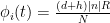
where d and h are death and hospitalization rates (again obtained from the CDC) for age category n, and |n| is the current size of or number of workers in n. N is the total size of the sector. What about R? Think of R for now as the estimated transmission rate. If R is greater than one, then it means that each infected/infectious person will spread the disease to at least one other person, probably more. If R is less than one, the disease dies out.
Perhaps the best way to show how this all works is to simulate it for an actual sector. Shown in these plots is the impact of the actual outbreak in March 2020, in San Francisco, for the Leisure and Hospitality sector (e.g. the hotel industry). We modeled the first 100 days of the outbreak, with an initial basic reproduction number, or R0, of 1.5. This value was derived from numerous data and model sources at the time that were being actively compiled by the California Department of Public Health’s California COVID Assessment Tool (CalCAT). Take a look at the plots below. The plot on the left shows the results of the SIR model, and the corresponding loss of employees in the sector during the same time period is shown in the plot on the right. Note the nonlinearity of the response: there is initially very little impact, but the acceleration is rapid as infection in the population ramps up. Things eventually settle down as the disease runs its course through the population. Importantly, the reduction of the number of employees is not a one to one match with the disease, and you can see this by comparing the Susceptible curve on the left, to the employment curve on the right. The lack of correspondence is driven by the fact that employment depends not only on illness in the Leisure and Hospitality sector, but also illness and changes of employment levels (and hence productivity and demand) in all the other sectors.
Finally, we can break this result down and examine each age category individually. We see immediately the uneven impact of the disease across age brackets, a result all too familiar as we witnessed the terrible impact that the pandemic has had on older people. The projected losses of employment for those 65 and older in the Leisure and Hospitality sector would be greater than 30%, even though they comprised only 7.7% of people employed in the sector.

In the next post we will look more broadly at the ten Californian SESs, and whereas here we looked at the impact on different age groups, next we will examine the impact on economies of different sizes and structure.

Pingback: COVID-19, Economics, Tipping Points – Economic Structure and Disease | Roopnarine's Food Weblog
Pingback: COVID-19, Economics, Tipping Points – Composition and Complexity | Roopnarine's Food Weblog